Demystifying the Central Limit Theorem

Marbles to the Rescue: Making the Abstract Tangible

Premise

Imagine that you have a bag filled with red and blue marbles.

How would you guess the proportion of red ones without going through every marble?

Simulating Marble Population

library(tidyverse)

source("../utils.R")   # helper functions

red_marble = "🔴"
blue_marble = "🔵"

# pretend you don't know this number
prob_red = 0.64
num_marbles = 1000

set.seed(42) 
marbles = sample(c(red_marble, blue_marble), 
                 size = num_marbles, 
                 replace = TRUE, 
                 prob = c(prob_red, 1 - prob_red))

Taking One Sample

set.seed(42)
one_sample = get_samples(marbles, sample_size = 10, number_of_samples = 1, func = is_red)

kable(one_sample, "html") |>
  kable_styling(font_size = 20)

sample_number	sample_value
1	0
1	1
1	1
1	0
1	1
1	1
1	0
1	1
1	0
1	0

sample_mean = mean(one_sample$sample_value)
print(str_glue("Percentage of red marbles: {sample_mean * 100}%"))

Percentage of red marbles: 50%

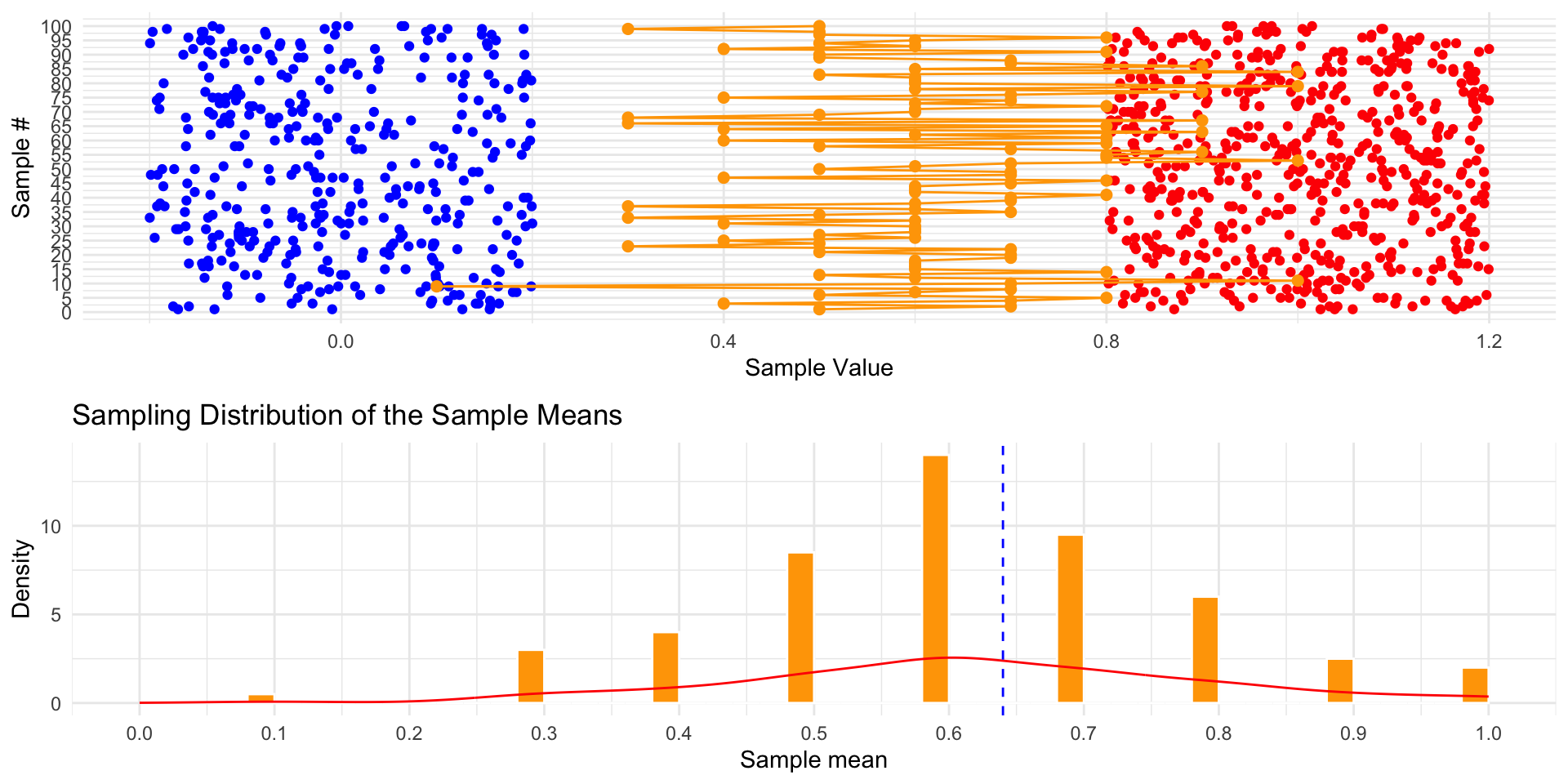
Taking More Samples

size = 10
n = 100

set.seed(42)
samples = get_samples(marbles, sample_size = size, number_of_samples = n, func = is_red)

sample_means = samples |>
  group_by(sample_number) |>
  summarise(proportion = mean(sample_value))

kable(head(sample_means, 5), "html") |>
  kable_styling(font_size = 20)

sample_number	proportion
1	0.5
2	0.7
3	0.4
4	0.7
5	0.8

standard_errors = tibble(sample_size = size, standard_error = sd(sample_means$proportion))
kable(standard_errors)

sample_size	standard_error
10	0.174298

Taking More Samples

p10 = plot_sample_means(samples, size, prob_red)
plot_samples_and_averages(samples, prob_red)

Increasing Sample Size to 20

size = 20
set.seed(42)
samples = get_samples(marbles, sample_size = size, number_of_samples = n, func = is_red)

sample_means = samples |>
  group_by(sample_number) |>
  summarise(proportion = mean(sample_value))

standard_errors = standard_errors |>
  add_row(sample_size = size, 
          standard_error = sd(sample_means$proportion))

kable(standard_errors)

sample_size	standard_error
10	0.1742980
20	0.1035665

Increasing Sample Size to 20

p20 = plot_sample_means(samples, size, prob_red)
grid.arrange(p10, p20, ncol=2)

Increasing Sample Size to 50

size = 50
set.seed(42)
samples = get_samples(marbles, sample_size = size, number_of_samples = n, func = is_red)

sample_means = samples |>
  group_by(sample_number) |>
  summarise(proportion = mean(sample_value))

standard_errors = standard_errors |>
  add_row(sample_size = size, 
          standard_error = sd(sample_means$proportion))

kable(standard_errors, "html")

sample_size	standard_error
10	0.1742980
20	0.1035665
50	0.0669916

Increasing Sample Size to 50

p50 = plot_sample_means(samples, size, prob_red)
grid.arrange(p10, p20, p50, ncol=2)

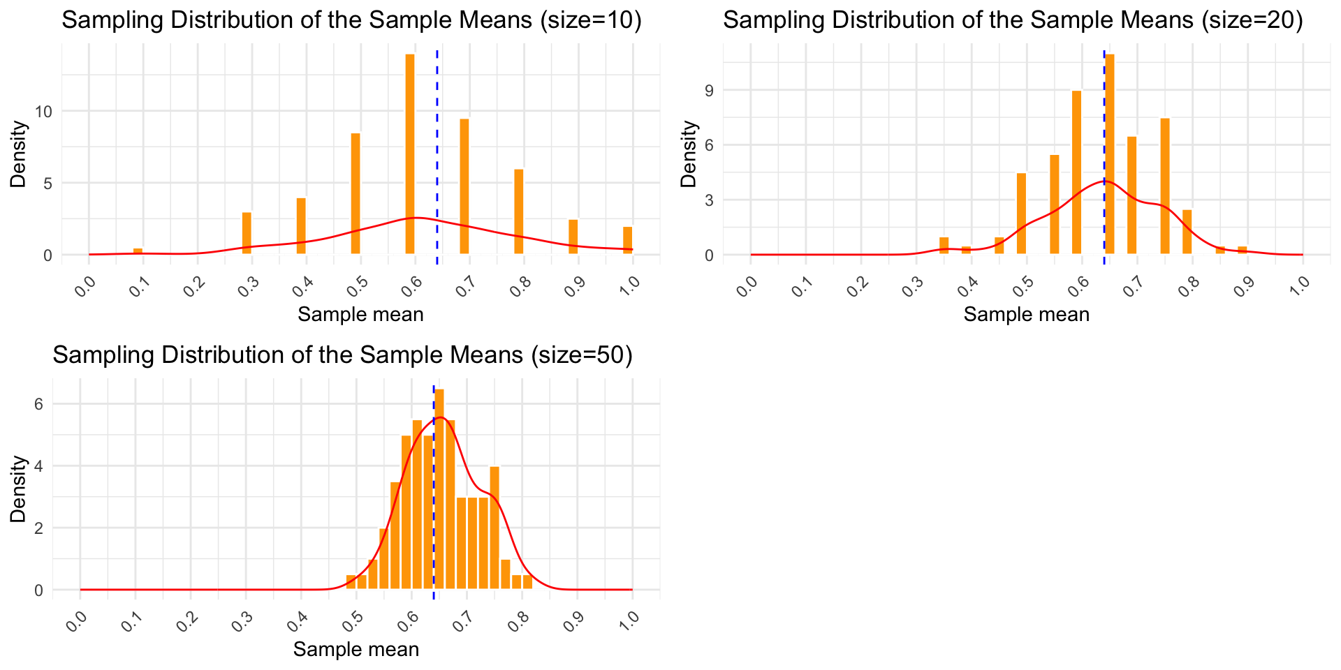
Increasing Sample Size to 100

size = 100
set.seed(42)
samples = get_samples(marbles, sample_size = size, number_of_samples = n, func = is_red)

sample_means = samples |>
  group_by(sample_number) |>
  summarise(proportion = mean(sample_value))

standard_errors = standard_errors |>
  add_row(sample_size = size, 
          standard_error = sd(sample_means$proportion))

kable(standard_errors, "html")

sample_size	standard_error
10	0.1742980
20	0.1035665
50	0.0669916
100	0.0494720

Increasing Sample Size to 100

p100 = plot_sample_means(samples, size, prob_red)
grid.arrange(p10, p20, p50, p100, ncol=2)

Central Limit Theorem

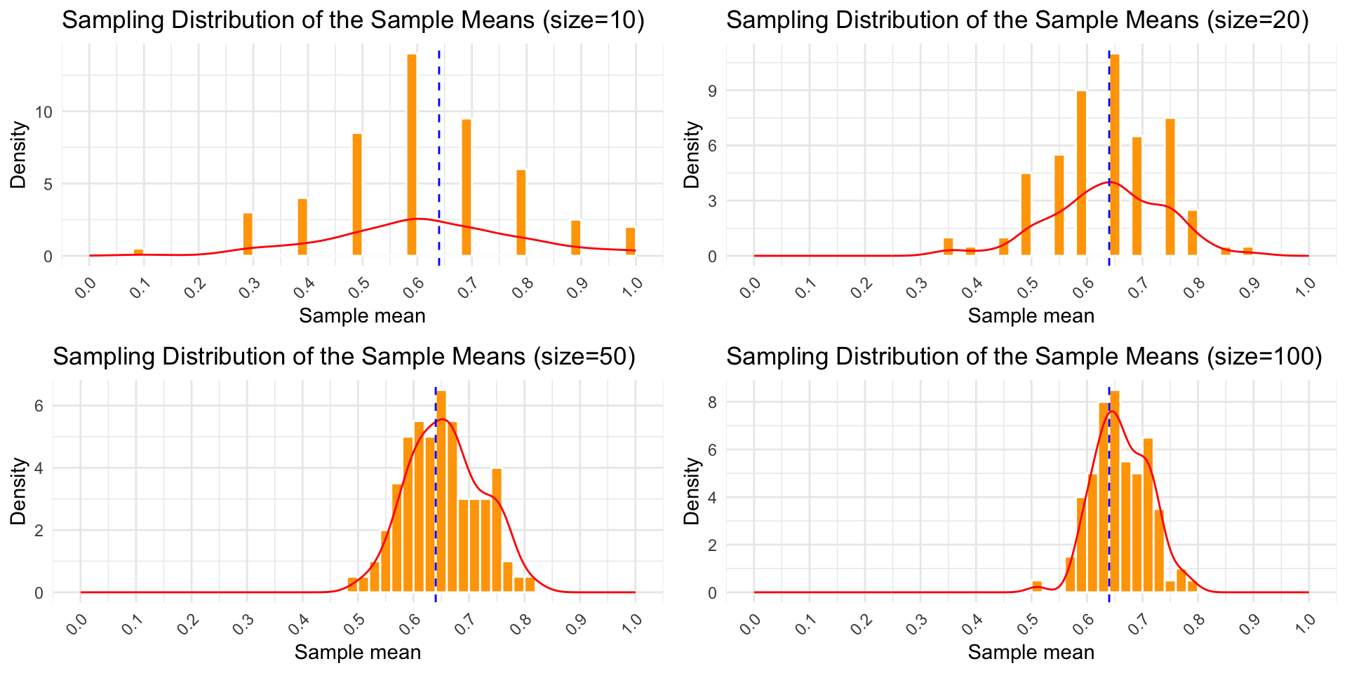
As the sample size increases, typically when it’s greater than 30, the distribution of the sample means approaches a normal distribution.

Skewed Data

set.seed(42)

n = 1000
mean_log = log(30000)
sd_log = 1 
salaries = rlnorm(n, meanlog = mean_log, sdlog = sd_log)

ggplot(data.frame(salaries), aes(x = salaries)) + 
  geom_histogram(bins = 50, fill = "blue", color = "black") + 
  geom_vline(xintercept = mean(salaries), color = "red", linewidth = 1) +
  geom_text(aes(x = mean(salaries) * 2, y = 400, label = str_glue("{round(mean(salaries), 2)}")), 
            color = "red", size = 3) +
  labs(title = "Salary Distribution", x = "Salary", y = "Count") + 
  theme_minimal()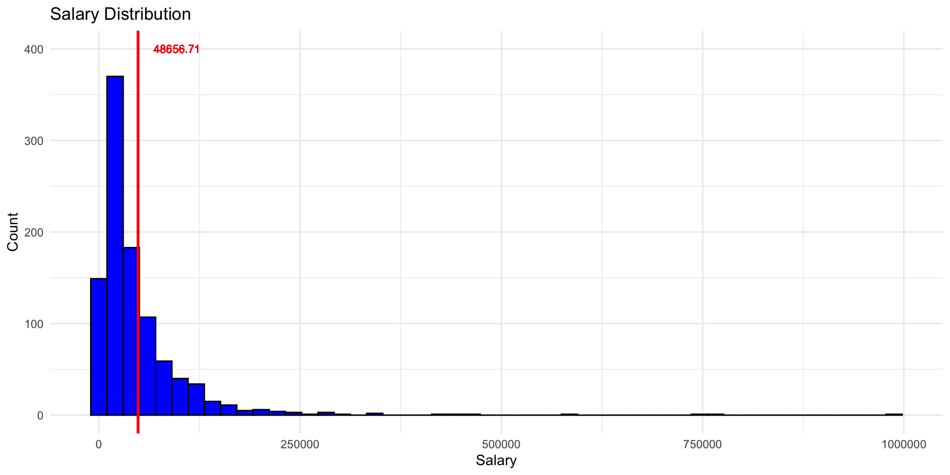

Skewed Data

samples = get_samples(salaries, sample_size = 100, number_of_samples = 100)
plot_samples_and_averages(samples, mean(salaries))

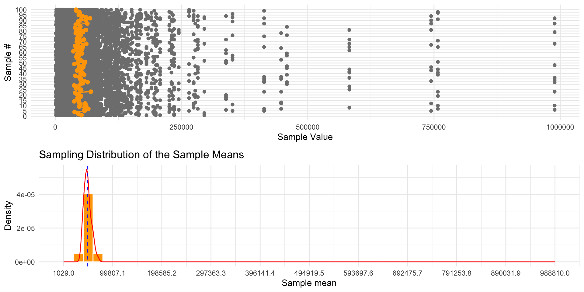
Key Insights

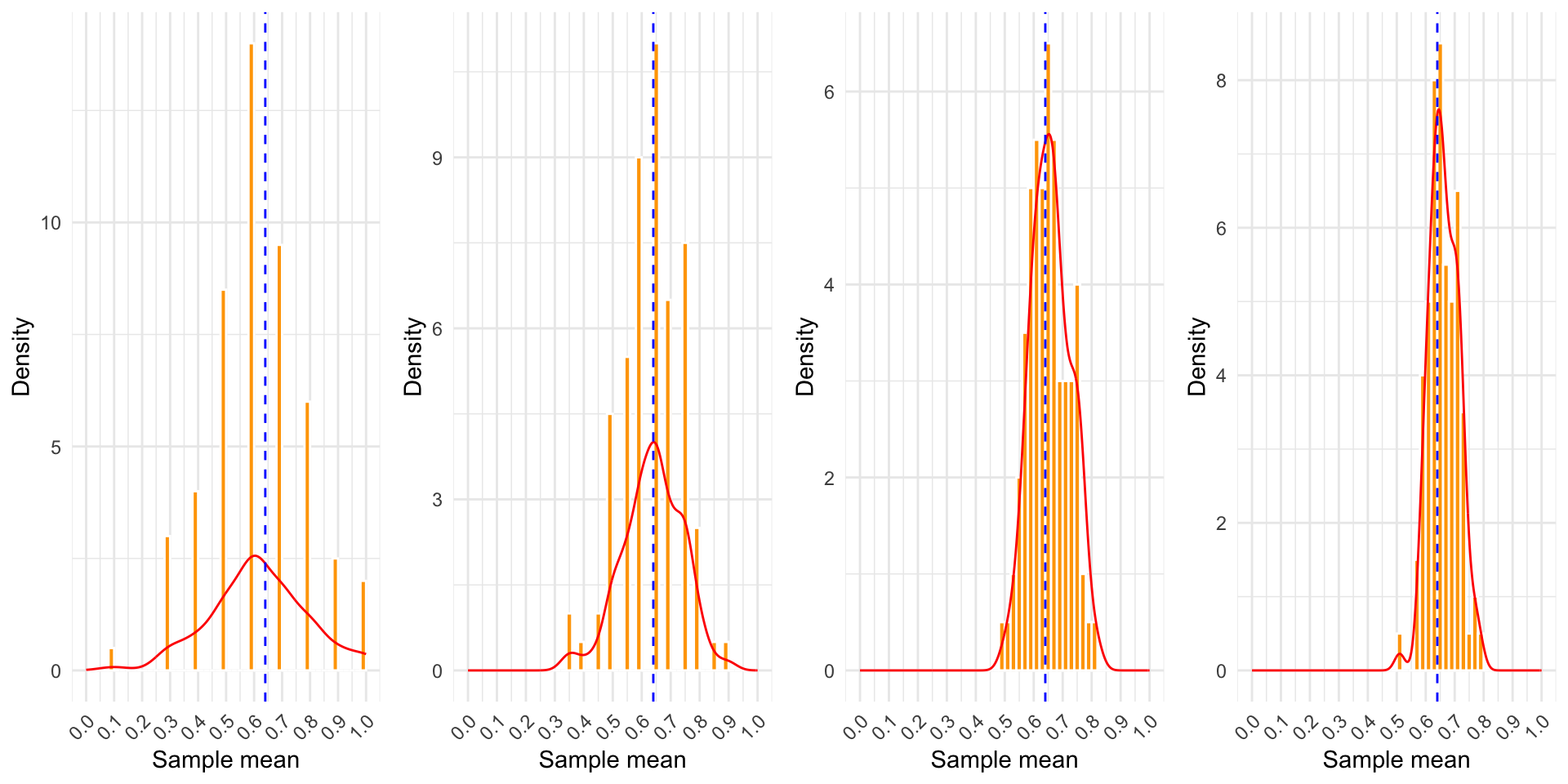
• Sample means cluster around the population mean
• Larger sample sizes decrease variability
• Distribution of sample means becomes more normal as size increases
• Works for any population distribution

Red Marble Proportion Estimation

set.seed(42)
one_sample = sample(marbles, 100)
print(str_glue("Percentage of red marbles: {mean(one_sample == red_marble) * 100}%"))

Percentage of red marbles: 60%

Question

• How confident are we in the estimation?
• How can we quantify our level of certainty?