Analysis of Variance (ANOVA)

How to compare means of more than two groups?

\(t\)-Test

• Sample size is small (\(n < 30\)) and/or population standard deviation is unknown.

\[t = \frac{\bar x - \mu}{s / \sqrt{n}} \sim t(n-1)\]

Three types of \(t\)-tests:

• One-sample \(t\)-test
• Two-sample \(t\)-test
• Paired \(t\)-test

Question:

• What if we want to compare the means of more than two groups?

Issues with Multiple \(t\)-Tests

• \(k \choose 2\) \(=\frac{k(k-1)}{2}\) pairwise \(t\)-tests

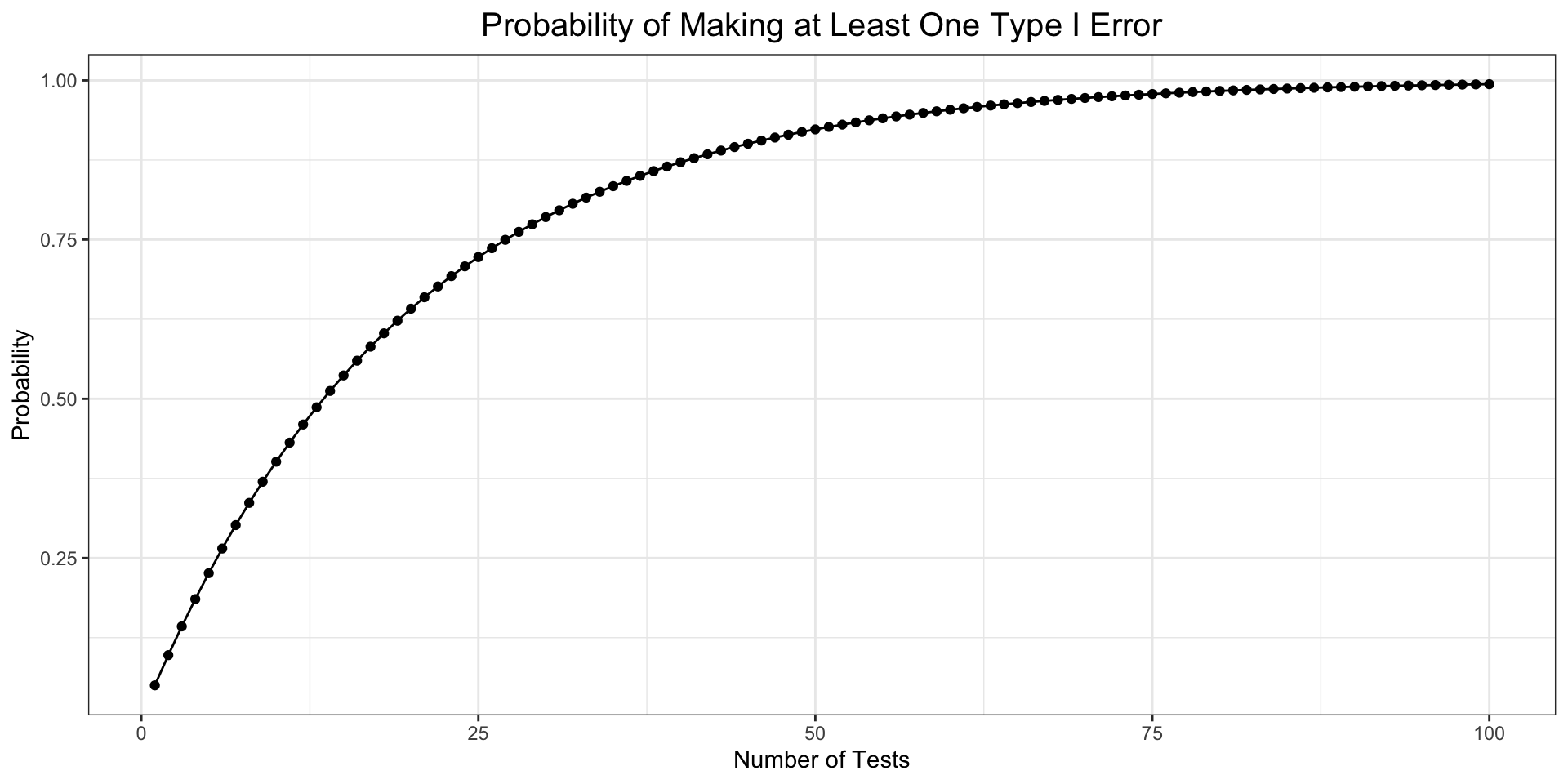
• The probability of making at least one Type I error is: \[P(\text{at least one Type I error}) = 1 - (1 - \alpha)^k\] where \(k\) is the number of tests.

Issues with Multiple \(t\)-Tests

Ways to Fix the Issues

• Bonferroni correction (\(\alpha_{new} = \frac{\alpha}{k}\), but can be overly conservative)
• Analysis of Variance (ANOVA)

Variance

• Variance measures the dispersion of a set of data points around their mean.
• Two kinds of variance in ANOVA:
  • Variance within groups: dispersion within each group
  • Variance between groups: dispersion between the group means
• ANOVA essentially compares the variation within groups against the variation between groups.

Intuition

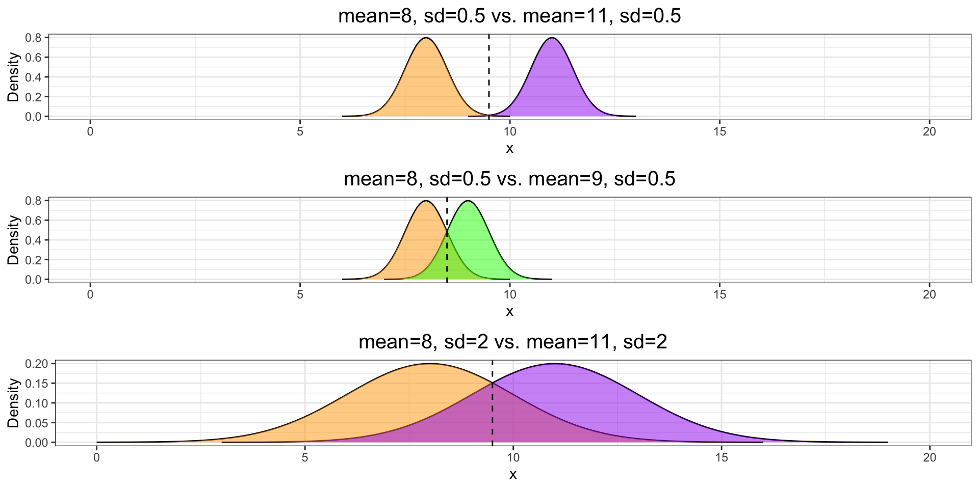
In which scenario are the means of the two groups significantly different?

Intuition

Between-group Variability

• The smaller the distance between sample means, the less likely population means will differ significantly. (Scenario 1 vs. Scenario 2)

Within-group Variability

• The greater the distance between sample means, the less likely population means will differ significantly. (Scenario 1 vs. Scenario 3)

Variance Between Groups

Sum of Squares Between

\[SS_{between} = \sum_{i=1}^{k} n_i (\bar{X}_i - \bar{X})^2\] where:

• \(k\) is the number of groups
• \(n_i\) is the number of observations in group \(i\)
• \(\bar{X}_i\) is the mean of group \(i\)
• \(\bar{X}\) is the overall mean

Variance Within Groups

Sum of Squares Within

\[SS_{within} = \sum_{i=1}^{k} \sum_{j=1}^{n_i} (X_{ij} - \bar{X}_i)^2\]

where:

• \(k\) is the number of groups
• \(n_i\) is the number of observations in group \(i\)
• \(\bar{X}_i\) is the mean of group \(i\)
• \(X_{ij}\) is the \(j\)th observation in group \(i\)

F-statistic

\[F = \frac{SS_{between} / (k - 1)}{SS_{within} / (N - k)} = \frac{MS_{between}}{MS_{within}} \sim F(k-1, N-k)\]

where \(N\) is the total number of observations and \(MS\) is the mean square.

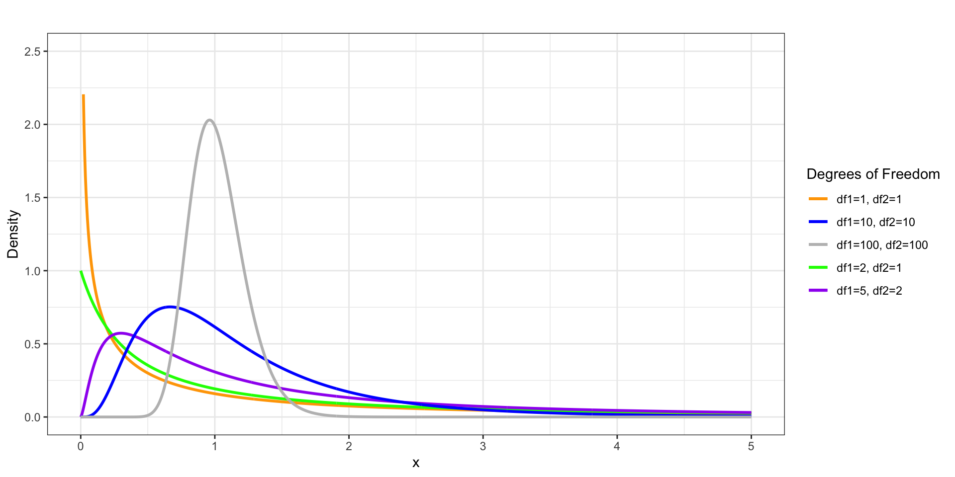
F-Distibution

Assumptions of ANOVA

• Independent and random samples
• Approximately normal population distribution
• Equal population variances (rule of thumb: \(\frac{\text{largest variance}}{\text{smallest variance}} < 2\))

Example

You’re testing the effect of three different call-to-action (CTA) button designs on your e-commerce website. The metric of interest is the click-through rate (CTR), which is the percentage of visitors who click the button. You randomly assign visitors to one of the three designs (A, B, or C) and record their CTRs.

• Design A: \(n_1 = 50, \bar x = 6.2, s = 0.5\)
• Design B: \(n_2 = 50, \bar x = 7.0, s = 0.5\)
• Design C: \(n_3 = 50, \bar x = 6.5, s = 0.5\)

Example

• \(H_0\): \(\mu_1 = \mu_2 = \mu_3\)
• \(H_a\): At least one \(\mu_i\) is different

set.seed(12345)
df = tibble(design_a = rnorm(50, 6.2, 0.5),
            design_b = rnorm(50, 7.0, 0.5),
            design_c = rnorm(50, 6.5, 0.5)) |>
  pivot_longer(cols = everything(), names_to = "design", values_to = "percentage")

result = aov(percentage ~ design, data = df)
summary(result)

             Df Sum Sq Mean Sq F value   Pr(>F)    
design        2  20.48  10.241   32.62 1.89e-12 ***
Residuals   147  46.15   0.314                     
---
Signif. codes:  0 '***' 0.001 '**' 0.01 '*' 0.05 '.' 0.1 ' ' 1

• Reject \(H_0\) at \(\alpha = 0.05\) significance level.
• We conclude that at least one of the designs has a different CTR.

Tukey’s HSD Test

• It can be used to determine which groups are different from each other.
• The test statistic is \(q = \frac{\bar x_i - \bar x_j}{\sqrt{MS_{within} / n}}\).
• The critical value is \(q_{\alpha, k, n-k}\).
• If \(|q| > q_{\alpha, k, n-k}\), then we reject \(H_0\) for the pair of groups.

TukeyHSD(result)

  Tukey multiple comparisons of means
    95% family-wise confidence level

Fit: aov(formula = percentage ~ design, data = df)

$design
                        diff         lwr        upr     p adj
design_b-design_a  0.8656309  0.60029322  1.1309687 0.0000000
design_c-design_a  0.2037145 -0.06162325  0.4690522 0.1673197
design_c-design_b -0.6619165 -0.92725419 -0.3965787 0.0000001

• We reject \(H_0\) for the pair of groups (A, B) and (B, C).
• We fail to reject \(H_0\) for the pair of groups (A, C).